Exploratory Data Analysis - Laptops market

The objective of this project is to analyze laptops’ prices based on their components, using exploratory data analysis tools. An appropriate data cleaning and EDA allows us to build high quality models and understand market context:

library(tidyverse)
library(DataExplorer)
library(stringr)
library(ggplot2)
library(rpart)
library(rpart.plot)
library(ggthemes)

laptop_raw <- read.csv("laptop_price.csv")
str(laptop_raw)

## 'data.frame':	1303 obs. of  13 variables:
##  $ laptop_ID       : int  1 2 3 4 5 6 7 8 9 10 ...
##  $ Company         : chr  "Apple" "Apple" "HP" "Apple" ...
##  $ Product         : chr  "MacBook Pro" "Macbook Air" "250 G6" "MacBook Pro" ...
##  $ TypeName        : chr  "Ultrabook" "Ultrabook" "Notebook" "Ultrabook" ...
##  $ Inches          : num  13.3 13.3 15.6 15.4 13.3 15.6 15.4 13.3 14 14 ...
##  $ ScreenResolution: chr  "IPS Panel Retina Display 2560x1600" "1440x900" "Full HD 1920x1080" "IPS Panel Retina Display 2880x1800" ...
##  $ Cpu             : chr  "Intel Core i5 2.3GHz" "Intel Core i5 1.8GHz" "Intel Core i5 7200U 2.5GHz" "Intel Core i7 2.7GHz" ...
##  $ Ram             : chr  "8GB" "8GB" "8GB" "16GB" ...
##  $ Memory          : chr  "128GB SSD" "128GB Flash Storage" "256GB SSD" "512GB SSD" ...
##  $ Gpu             : chr  "Intel Iris Plus Graphics 640" "Intel HD Graphics 6000" "Intel HD Graphics 620" "AMD Radeon Pro 455" ...
##  $ OpSys           : chr  "macOS" "macOS" "No OS" "macOS" ...
##  $ Weight          : chr  "1.37kg" "1.34kg" "1.86kg" "1.83kg" ...
##  $ Price_euros     : num  1340 899 575 2537 1804 ...

head(laptop_raw)

##   laptop_ID Company     Product  TypeName Inches
## 1         1   Apple MacBook Pro Ultrabook   13.3
## 2         2   Apple Macbook Air Ultrabook   13.3
## 3         3      HP      250 G6  Notebook   15.6
## 4         4   Apple MacBook Pro Ultrabook   15.4
## 5         5   Apple MacBook Pro Ultrabook   13.3
## 6         6    Acer    Aspire 3  Notebook   15.6
##                     ScreenResolution                        Cpu  Ram
## 1 IPS Panel Retina Display 2560x1600       Intel Core i5 2.3GHz  8GB
## 2                           1440x900       Intel Core i5 1.8GHz  8GB
## 3                  Full HD 1920x1080 Intel Core i5 7200U 2.5GHz  8GB
## 4 IPS Panel Retina Display 2880x1800       Intel Core i7 2.7GHz 16GB
## 5 IPS Panel Retina Display 2560x1600       Intel Core i5 3.1GHz  8GB
## 6                           1366x768    AMD A9-Series 9420 3GHz  4GB
##                Memory                          Gpu      OpSys Weight
## 1           128GB SSD Intel Iris Plus Graphics 640      macOS 1.37kg
## 2 128GB Flash Storage       Intel HD Graphics 6000      macOS 1.34kg
## 3           256GB SSD        Intel HD Graphics 620      No OS 1.86kg
## 4           512GB SSD           AMD Radeon Pro 455      macOS 1.83kg
## 5           256GB SSD Intel Iris Plus Graphics 650      macOS 1.37kg
## 6           500GB HDD                AMD Radeon R5 Windows 10  2.1kg
##   Price_euros
## 1     1339.69
## 2      898.94
## 3      575.00
## 4     2537.45
## 5     1803.60
## 6      400.00

Our original file contains around 1303 records, described in 13 variables. The variables are listed below, the majority are categorical. Our target variable in this project is “price_euros”.

laptop_ID
Company
Product
TypeName
Inches
ScreenResolution
Cpu
Ram
Memory
Gpu
OpSys
Weight
Price_euros

Data preprocessing

I applied some techniques to check the quality of the data and make the necessary transformations:

The are no missing values in our dataset.
I extracted numeric data from variables like Screen_Resolution, Ram, Memory and Weight. Also, we transformed into numeric types the screen_resolution and weight.
I grouped some categorical variables, like CPU and GPU, in the principal models.
I checked for other data types.

plot_intro(laptop_raw)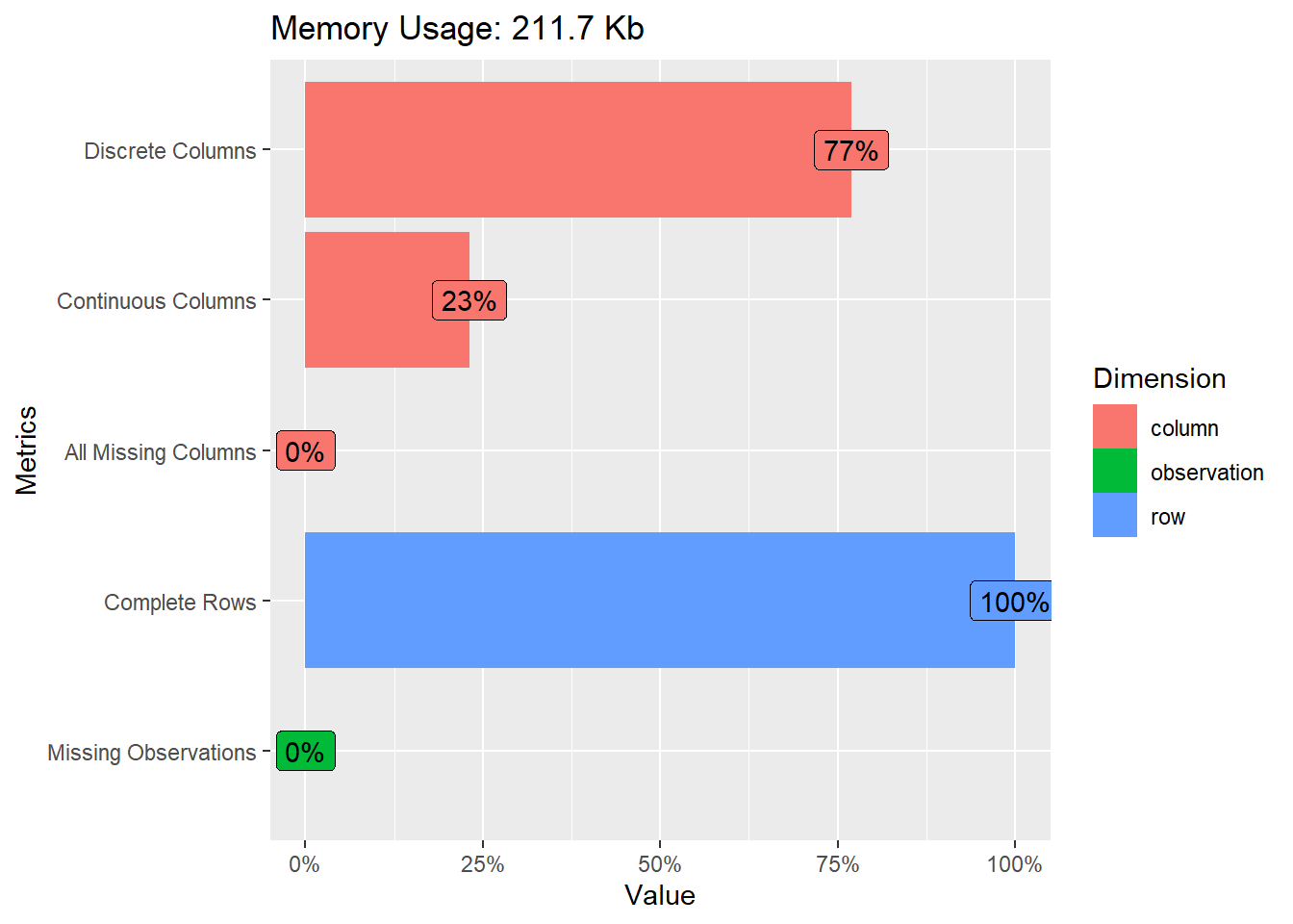

laptop_cl <- laptop_raw %>%
  rename_with(tolower, everything()) %>%
  transmute(
    laptop_id,
    company,
    product,
    typename,
    inches = case_when(
      inches < 14 ~ "<14",
      inches >= 14 & inches <= 16 ~ "14-16",
      inches > 16 ~ ">16",
    ),
    screen_res = str_extract(screenresolution, "\\b\\d{3,4}x\\d{3,4}\\b"),
    cpu = case_when(
      str_detect(cpu, fixed("Intel Core i7")) ~ "Intel Core i7",
      str_detect(cpu, fixed("Intel Core i5")) ~ "Intel Core i5",
      str_detect(cpu, fixed("Intel Core i3")) ~ "Intel Core i3",
      str_detect(cpu, "Intel") ~ "Intel other",
      str_detect(cpu, fixed("AMD")) ~ "AMD",
      TRUE ~ "other"
    ),
    ram = str_extract(ram, "\\d*"),
    gpu = case_when(
      str_detect(gpu, fixed("Intel")) ~ "Intel Graphics",
      str_detect(gpu, fixed("Nvidia GeForce")) ~ "Nvidia GeForce",
      str_detect(gpu, "Quadro|GTX") ~ "Nvidia Quadro/GTX",
      str_detect(gpu, fixed("ARM")) ~ "ARM",
      str_detect(gpu, fixed("AMD")) ~ "AMD",
      TRUE ~ "other"
    ),
    op_sys = opsys,
    weight = as.numeric(str_extract(weight, "\\d+\\.?\\d*")),
    price_euros
  )

memory_cl <- laptop_raw %>%
  separate(Memory, c("memorySSD", "memoryHDD"), sep = "\\+") %>%
  mutate(
    memoryx = laptop_raw$Memory,
    memorySSD = as.numeric(str_extract(memorySSD, "\\d*")),
    memoryHDD = as.numeric(str_extract(memoryHDD, "\\d+")),
  ) %>%
  mutate(
    memorySSD = replace(memorySSD, memorySSD == 1, 1000),
    memorySSD = replace(memorySSD, memorySSD == 2, 2000),
    memoryHDD = replace(memoryHDD, memoryHDD == 1, 1000),
    memoryHDD = replace(memoryHDD, memoryHDD == 2, 2000),
    memoryHDD = replace_na(memoryHDD, 0),
    totalmemory = memorySSD + memoryHDD
  ) %>%
  dplyr::select(c(laptop_ID, totalmemory))

laptop_cl <- laptop_cl %>%
  dplyr::left_join(memory_cl, by = c("laptop_id" = "laptop_ID")) %>%
  mutate(
    totalmemory = as.character(totalmemory)
  )

head(laptop_cl)

##   laptop_id company     product  typename inches screen_res           cpu ram
## 1         1   Apple MacBook Pro Ultrabook    <14  2560x1600 Intel Core i5   8
## 2         2   Apple Macbook Air Ultrabook    <14   1440x900 Intel Core i5   8
## 3         3      HP      250 G6  Notebook  14-16  1920x1080 Intel Core i5   8
## 4         4   Apple MacBook Pro Ultrabook  14-16  2880x1800 Intel Core i7  16
## 5         5   Apple MacBook Pro Ultrabook    <14  2560x1600 Intel Core i5   8
## 6         6    Acer    Aspire 3  Notebook  14-16   1366x768           AMD   4
##              gpu     op_sys weight price_euros totalmemory
## 1 Intel Graphics      macOS   1.37     1339.69         128
## 2 Intel Graphics      macOS   1.34      898.94         128
## 3 Intel Graphics      No OS   1.86      575.00         256
## 4            AMD      macOS   1.83     2537.45         512
## 5 Intel Graphics      macOS   1.37     1803.60         256
## 6            AMD Windows 10   2.10      400.00         500

# convert character variables to factors
laptop_fr <- laptop_cl %>%
  dplyr::select(-laptop_id) %>%
  mutate(across(where(is.character), factor))

head(laptop_fr)

##   company     product  typename inches screen_res           cpu ram
## 1   Apple MacBook Pro Ultrabook    <14  2560x1600 Intel Core i5   8
## 2   Apple Macbook Air Ultrabook    <14   1440x900 Intel Core i5   8
## 3      HP      250 G6  Notebook  14-16  1920x1080 Intel Core i5   8
## 4   Apple MacBook Pro Ultrabook  14-16  2880x1800 Intel Core i7  16
## 5   Apple MacBook Pro Ultrabook    <14  2560x1600 Intel Core i5   8
## 6    Acer    Aspire 3  Notebook  14-16   1366x768           AMD   4
##              gpu     op_sys weight price_euros totalmemory
## 1 Intel Graphics      macOS   1.37     1339.69         128
## 2 Intel Graphics      macOS   1.34      898.94         128
## 3 Intel Graphics      No OS   1.86      575.00         256
## 4            AMD      macOS   1.83     2537.45         512
## 5 Intel Graphics      macOS   1.37     1803.60         256
## 6            AMD Windows 10   2.10      400.00         500

Exploratory Analysis

laptop_fr %>%
  ggplot(aes(price_euros, fct_reorder(ram, price_euros))) +
  geom_boxplot() +
  labs(y = "", x = "", title = "Price (€) by Ram capacity") +
  theme_classic()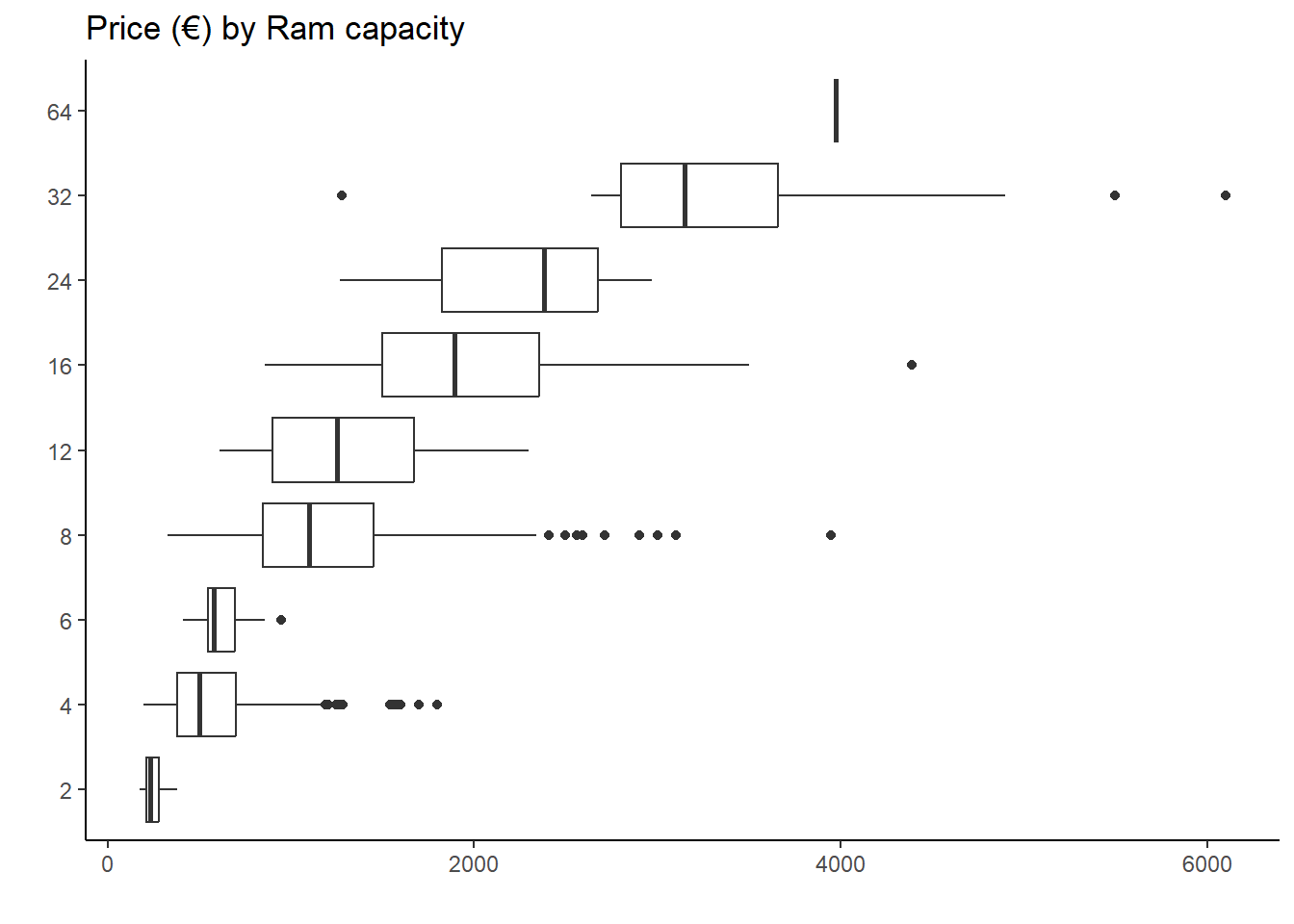

RAM: the boxplot of RAM versus price shows the distribution of prices for laptops with different amounts of RAM. We see that laptops with higher RAM capacity have a higher median price than laptops with lower RAM capacity.

laptop_fr %>%
  ggplot(aes(price_euros, fct_reorder(cpu, price_euros))) +
  geom_boxplot() +
  labs(y = "", x = "", title = "Price (€) by CPU type") +
  theme_classic()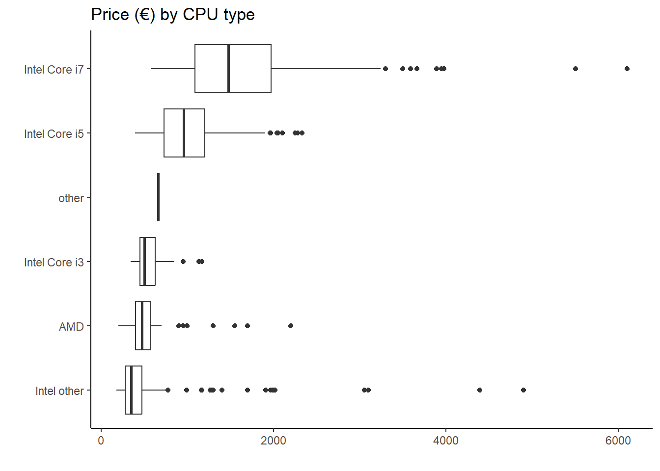

laptop_fr %>%
  ggplot(aes(price_euros, fct_reorder(gpu, price_euros))) +
  geom_boxplot() +
  labs(y = "", x = "", title = "Price (€) by GPU type") +
  theme_classic()

CPU/GPU: the boxplot of CPU and GPU versus price would show the distribution of prices for laptops with different processor types. We see that laptops with higher-quality processors have a higher median price than laptops with lower-quality processors.

laptop_fr %>%
  ggplot(aes(price_euros, fct_reorder(inches, price_euros))) +
  geom_boxplot() +
  labs(y = "", x = "", title = "Price (€) by Screen size (inches)") +
  theme_classic()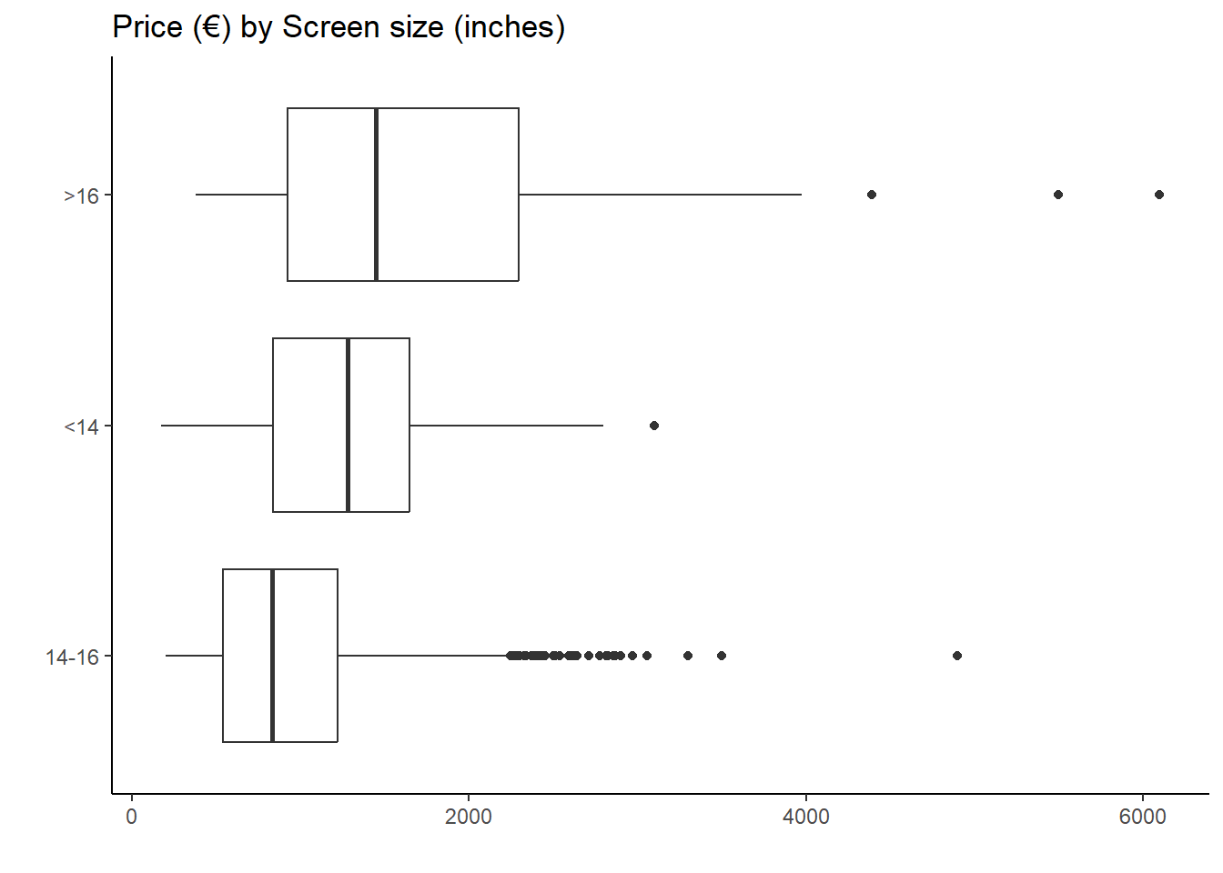

Screen size: the boxplot of inches versus price shows the distribution of prices for laptops with different screen sizes. We observe that laptops with larger screen sizes have a higher median price than laptops with smaller screen sizes.

laptop_fr %>%
  ggplot(aes(price_euros, fct_reorder(totalmemory, price_euros))) +
  geom_boxplot() +
  labs(y = "", x = "", title = "Price (€) by Memory capacity") +
  theme_classic()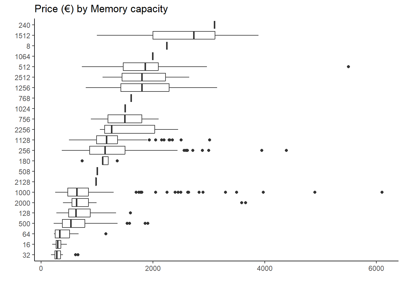

Memory: the boxplot of memory versus price shows the distribution of prices for laptops with different storage capacities. We see that not always laptops with larger storage capacity would have a higher median price than laptops with smaller storage capacity, because the total capacity combines two technologies (HDD and SSD), and probable laptops with SSD have higher prices.

laptop_fr %>%
  ggplot(aes(price_euros, fct_reorder(op_sys, price_euros))) +
  geom_boxplot() +
  labs(y = "", x = "", title = "Price (€) by Operative system") +
  theme_classic()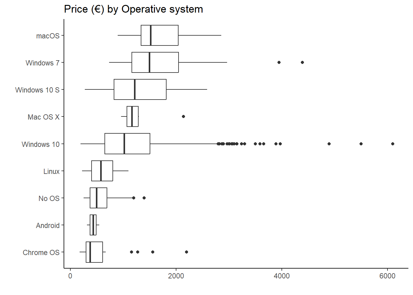

laptop_fr %>%
  ggplot(aes(price_euros, fct_reorder(company, price_euros))) +
  geom_boxplot() +
  labs(y = "", x = "", title = "Price (€) by Company") +
  theme_classic()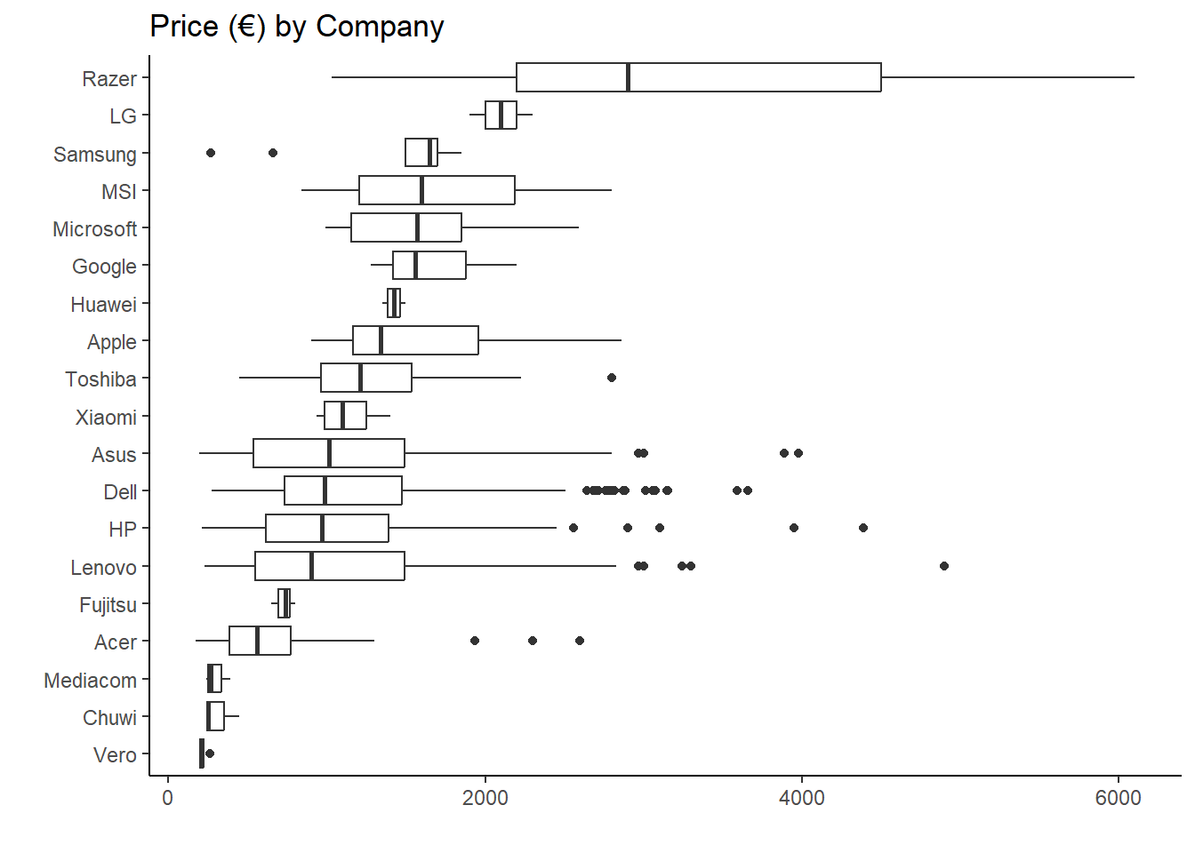

Based on the boxplots of different laptop components versus price, we can suggest that there are positive correlations between the predictors and the price, laptops with better components tend to have a higher price. We can verify this hypothesis with an ANOVA test. In terms of RAM, I confirmed the alternative hypothesis, because of the p-value of the test.

res.aov <- aov(price_euros ~ ram, data = laptop_fr)
summary(res.aov)

##               Df    Sum Sq  Mean Sq F value Pr(>F)    
## ram            8 375624250 46953031   233.2 <2e-16 ***
## Residuals   1294 260550712   201353                   
## ---
## Signif. codes:  0 '***' 0.001 '**' 0.01 '*' 0.05 '.' 0.1 ' ' 1

laptop_fr %>%
  ggplot(aes(price_euros)) +
  geom_histogram(bins = 13) +
  labs(y = "", x = "", title = "Laptops' price (€) distributon") +
  theme_minimal()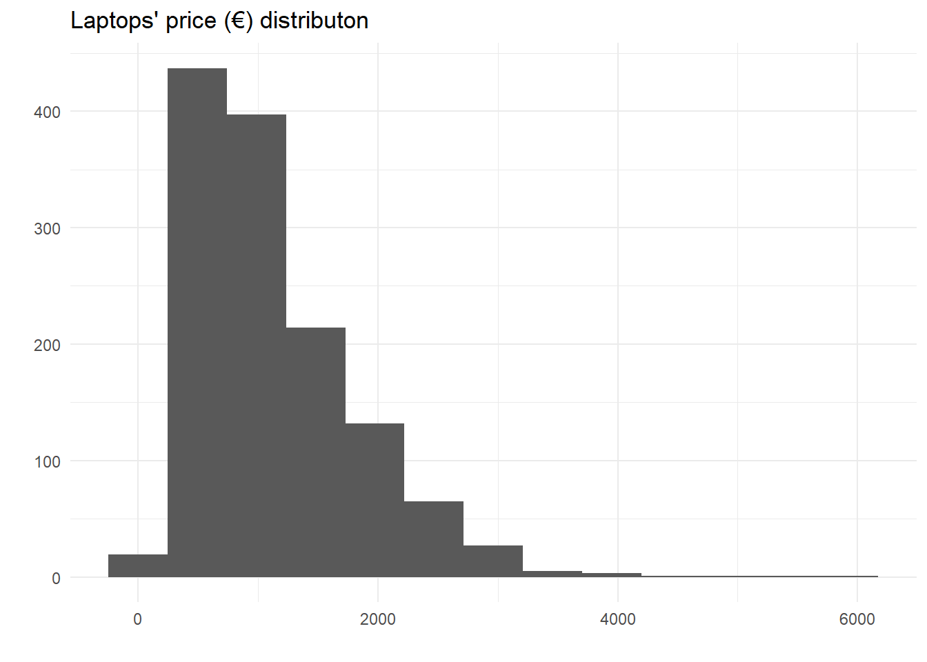

laptop_fr %>% ggplot(aes(y = price_euros)) +
  geom_boxplot() +
  labs(y = "", x = "", title = "Laptops' price (€) distribution") +
  theme_minimal()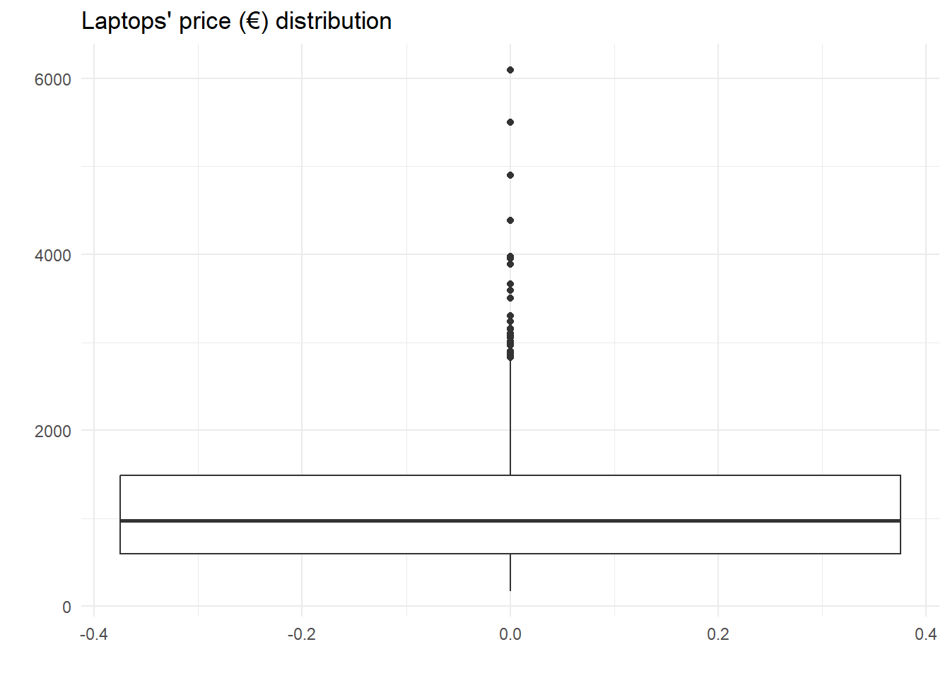

Analyzing our target variable we realized that it has a right-skewed distribution, it means that the data is not symmetrically distributed around its mean, but rather has a long tail towards the right side of the distribution, with a concentration of lower values towards the left side. The implications of this is that the mean of the variable is higher than the median, and the standard deviation may not accurately reflect the spread of the data. In addition, it can cause some modeling techniques, such as linear regression, to perform poorly because it assumes that the target variable has a normal distribution.

GitHub