Energy demand forecasting using time series

Accurate demand forecasting is crucial for businesses to make informed decisions, optimize inventory levels, and improve customer satisfaction. By leveraging time series models like ARIMA and Prophet, businesses can not only predict demand but also identify trends and patterns to develop proactive strategies.
Arima
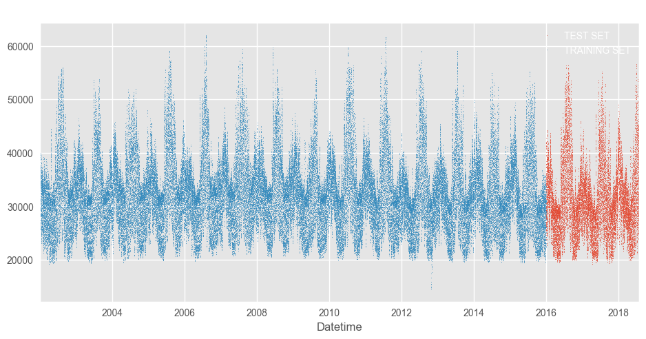
To begin with, the dataset is prepared by loading the data and replacing the index with the corresponding date. Then, the dataset is split into training and testing subsets.
import pandas as pd
import numpy as np
import matplotlib.pyplot as plt
import statsmodels.api as sm
import statsmodels.formula.api as smf
from prophet import Prophet
from sklearn.metrics import mean_squared_error
from statsmodels.tsa.arima.model import ARIMA
plt.style.use('ggplot')
plt.style.use('fast')
df_arima = pd.read_csv("PJME_hourly.csv")
df_arima.Datetime = pd.DatetimeIndex(df_arima.Datetime)
df_arima = df_arima.reset_index(drop=True)
df_arima.index = pd.PeriodIndex(df_arima.Datetime, freq='H')
df_arima = df_arima.drop(df_arima.columns[0], axis=1)
df_arima
| PJME_MW | |
|---|---|
| Datetime | |
| 2002-12-31 01:00 | 26498.0 |
| 2002-12-31 02:00 | 25147.0 |
| 2002-12-31 03:00 | 24574.0 |
| 2002-12-31 04:00 | 24393.0 |
| 2002-12-31 05:00 | 24860.0 |
| … | … |
| 2018-01-01 20:00 | 44284.0 |
| 2018-01-01 21:00 | 43751.0 |
| 2018-01-01 22:00 | 42402.0 |
| 2018-01-01 23:00 | 40164.0 |
| 2018-01-02 00:00 | 38608.0 |
split_point = '1-Jan-2016'
train_arima = df_arima.loc[df_arima.index < split_point].copy()
test_arima= df_arima.loc[df_arima.index >= split_point].copy()

test_arima \
    .rename(columns={'PJME_MW': 'TEST SET'}) \
    .join(train_arima.rename(columns={'PJME_MW': 'TRAINING SET'}),
          how='outer') \
    .plot(figsize=(10, 5), title='Energy Consumption (MW)', style='.', ms=1)
plt.show()

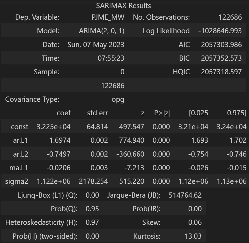
Now, the ARIMA model is fitted, defining the p,d, and q parameters:
model_arima = ARIMA(train_arima, order=(2,0,1))
model_arima_fit = model_arima.fit()
model_arima_fit.summary()

The performance of the ARIMA model is evaluated on the testing set. The model’s predictive accuracy is then quantified using error metrics, resulting in a MAPE of 17%.
arima_forecast = model_arima_fit.predict(start=len(train_arima), end=len(df_arima)-1, dynamic=False)
arima_forecast = pd.DataFrame(arima_forecast)

# RMSE
np.sqrt(mean_squared_error(y_true=test_arima['PJME_MW'],
                   y_pred=arima_forecast['predicted_mean']))
6474.90208717094
#MAPE
def mape(y_true, y_pred):
    y_true, y_pred = np.array(y_true), np.array(y_pred)
    return np.mean(np.abs((y_true - y_pred) / y_true)) * 100

mape(y_true=test_arima['PJME_MW'],
                   y_pred=arima_forecast['predicted_mean'])
17.475612965761343
PROPHET
To enhance our predictions, we leverage the time series prediction tool, Prophet, developed by Facebook. To use Prophet, we need to format our columns to comply with the required naming conventions.
df = pd.read_csv("PJME_hourly.csv", index_col=[0],
                  parse_dates=[0])
df_train = df.loc[df.index < split_point].copy()
df_test = df.loc[df.index >= split_point].copy()

train_prophet = df_train.reset_index() \
    .rename(columns={'Datetime':'ds', 'PJME_MW':'y'})
test_prophet = df_test.reset_index() \
    .rename(columns={'Datetime':'ds', 'PJME_MW':'y'})
The model is instantiated, trained, and applied to make predictions on the testing set:
model = Prophet()
model.fit(train_prophet)
prophet_forecast = model.predict(test_prophet)
prophet_forecast.loc[:,['ds','yhat_lower','yhat_upper','trend']]
| ds | yhat_lower | yhat_upper | yhat | trend | |
|---|---|---|---|---|---|
| 0 | 2016-01-01 00:00:00 | 25246.750720 | 34505.876842 | 30003.037051 | 31217.898672 |
| 1 | 2016-01-01 01:00:00 | 23586.638059 | 32278.979065 | 27986.257615 | 31217.867138 |
| 2 | 2016-01-01 02:00:00 | 21633.009369 | 31055.358356 | 26485.508878 | 31217.835604 |
| 3 | 2016-01-01 03:00:00 | 21036.939515 | 30026.875296 | 25613.179301 | 31217.804070 |
| 4 | 2016-01-01 04:00:00 | 21334.493617 | 30091.451316 | 25468.367381 | 31217.772536 |
| … | … | … | … | … | … |
| 22675 | 2018-08-02 20:00:00 | 23131.497863 | 62687.692651 | 41691.940934 | 30502.835532 |
| 22676 | 2018-08-02 21:00:00 | 21486.832495 | 61935.114453 | 40912.203071 | 30502.803998 |
| 22677 | 2018-08-02 22:00:00 | 20676.075026 | 61192.507108 | 39282.961743 | 30502.772464 |
| 22678 | 2018-08-02 23:00:00 | 17708.112800 | 58683.494409 | 37083.837882 | 30502.740930 |
| 22679 | 2018-08-03 00:00:00 | 15315.390736 | 57082.285941 | 34772.081648 | 30502.709396 |
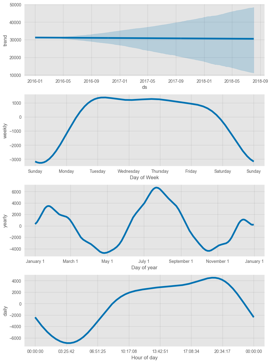
Upon comparing the forecasts to the actual values, it can be observed that the model follows the behavior of the original time series. Furthermore, the components plot reveals the underlying patterns and trends for each of the main time units, including weekly, yearly, and hourly.
f, ax = plt.subplots(figsize=(15, 5))
ax.scatter(df_test.index, df_test['PJME_MW'], color='violet')
fig = model.plot(prophet_forecast, ax=ax)

fig = model.plot_components(prophet_forecast)
plt.show()

The evaluation of the Prophet model is performed using the RMSE and MAPE metrics. The model exhibits better performance compared to the ARIMA model, with a lower MAPE error of 15.8%. Indeed, a basic Prophet model is effective in predicting energy demand.
# RMSE
np.sqrt(mean_squared_error(y_true=df_test['PJME_MW'],
                   y_pred=prophet_forecast['yhat']))
6307.621116334434
#MAPE
mape(y_true=df_test['PJME_MW'],
                   y_pred=prophet_forecast['yhat'])
15.838310394639882
