ML and statistical classification models

1. Case Description
This project aims to develop a classification model using supervised learning techniques to identify energy-efficient buildings in New York City. The dataset used for this project is provided by NYC Open Data and consists of reports on more than 29,000 buildings and 254 features for the calendar year 2019. The identification of energy-efficient buildings is crucial for achieving NYC’s ambitious goal of 100% carbon-free electricity and reducing emissions by 2040. This model will aid in benchmarking and achieving decarbonization goals.
library(tidyverse)
library(ggplot2)
library(DataExplorer)
library(caret)
library(forcats)
library(factoextra)
library(cluster)
library(mclust)
library(GGally)
library(plotly)
library(sf)
library(rnaturalearth)
library(rnaturalearthdata)
library(ggthemes)
library(pROC)
library(sjPlot)
data = read.csv("Energy_and_Water_Data_Disclosure_for_Local_Law_84_2020__Data_for_Calendar_Year_2019_.csv")
2. Cleaning and Feature Engineering
We started cleaning the dataset and making some feature selection, in order to choose the relevant variables for our analysis. During the process, we changed the data type of all variables to integer, and the NAs were dropped.
In addition, we do some feature engineering. In order to build comparable variables that are computed as total volumes, we divided them by the size of the buildings. As a result, we achieve a subset of 13 variables and more than 2500 observations. We didn’t include more features because many of the original variables were disaggregated measures of those that we chose.
Our final features are listed below:
- Energy-Star Score
- Occupancy per m^2: People/ft^2
- Weather Normalized Source Energy Use Intensity (EUI): kBtu/ft^2
- Fuel Oil Use: kBtu/ft^2
- Weather Normalized Site Natural Gas Use: therms/ft^2
- Weather Normalized Site Grid Purchased Electricity: kWh/ft^2
- Electricity Use, generated from Onsite Renewable Systems: kWh/ft^2
- Total GHG Emissions: Metric Tons CO2e/ft^2
- Water Use Intensity All Water Sources (WUI): gal/ft^2
- Gross Floor Area: ft^2
- Use type
- Longitude
- Latitude
building_type = data %>% select(Property.Id, Largest.Property.Use.Type)

clean_ny = data %>%
  # feature selection
  select(c(Largest.Property.Use.Type...Gross.Floor.Area..ft..,
          ENERGY.STAR.Score, Occupancy,
          Weather.Normalized.Source.EUI..kBtu.ft..,
           Weather.Normalized.Source.Energy.Use..kBtu., Fuel.Oil..2.Use..kBtu.,
           Weather.Normalized.Site.Natural.Gas.Use..therms.,
           Weather.Normalized.Site.Electricity..kWh.,
           Electricity.Use...Grid.Purchase.and.Generated.from.Onsite.Renewable.Systems..kWh.,
           Total.GHG.Emissions..Metric.Tons.CO2e.,  Water.Use..All.Water.Sources...kgal.,
           Water.Use.Intensity..All.Water.Sources...gal.ft.., Property.Id,
           Latitude,
           Longitude
           )) %>%
  mutate(across(where(is.character), as.integer)) %>%
  # Discarting NAs
  drop_na() %>%
  #Renaming variables
  rename(area = 1,
         energy_score = 2,
         occupancy = 3,
         eui = 4,
         energy_use = 5,
         fueloil_use = 6,
         gas_use = 7,
         electricity_grid_use = 8,
         renewables_use = 9,
         ghg_emissions = 10,
         water_use = 11,
         wui = 12
         ) %>%
  # Feature engineering
  mutate(
    occupancy_pa = occupancy/area,
    fueloil_use_pa = fueloil_use/area,
    gas_use_pa = gas_use/area,
    electricity_useGP_pa = electricity_grid_use/area,
    renewables_use_pa = renewables_use/area,
    ghg_emissions_pa = ghg_emissions/area,
  ) %>%
  select(!c(energy_use, water_use, occupancy, fueloil_use,gas_use,electricity_grid_use,renewables_use, ghg_emissions)) %>%
  left_join(building_type, by = 'Property.Id' ) %>%
  rename(type = Largest.Property.Use.Type) %>%
  mutate(type = as.factor(type)) %>%
  distinct()

head(clean_ny)
| area | energy_score | eui | wui | Property.Id | Latitude | Longitude |
|---|---|---|---|---|---|---|
| 308789 | 38 | 469 | 79 | 28404 | 40.87239 | -73.91267 |
| 885474 | 66 | 147 | 4 | 1143922 | 40.70455 | -74.00664 |
| 1852980 | 92 | 105 | 11 | 1143934 | 40.72066 | -74.01010 |
| 1414803 | 67 | 160 | 14 | 1409171 | 40.74670 | -73.94348 |
| 437571 | 96 | 80 | 4 | 1409173 | 40.74757 | -73.94352 |
| 171725 | 90 | 79 | 48 | 1633012 | 40.83590 | -73.89046 |
| occupancy_pa | fueloil_use_pa | gas_use_pa | electricity_useGP_pa | renewables_use_pa | ghg_emissions_pa | type |
| 3.238457e-04 | 0.00000000 | 1.619908740 | 31.366687 | 31.750652 | 0.017212401 | Hospital |
| 6.776032e-05 | 0.00000000 | 0.000000000 | 11.655381 | 11.655385 | 0.005346289 | Office |
| 5.396712e-05 | 0.03068355 | 0.190909238 | 8.750489 | 8.750488 | 0.003669225 | Office |
| 7.068122e-05 | 0.00000000 | 0.002825835 | 16.994128 | 17.150692 | 0.004970303 | Office |
| 2.285343e-04 | 1.16847323 | 0.071743786 | 9.215922 | 9.215924 | 0.003128635 | Office |
| 5.823264e-04 | 5.18971029 | 0.369474450 | 3.739147 | 3.745523 | 0.003371670 | K-12 School |
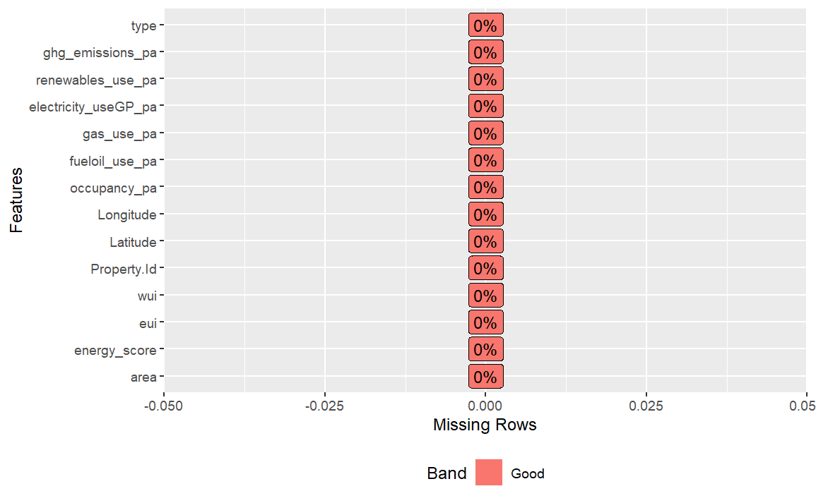
plot_missing(clean_ny)
3. Exploratory Analysis
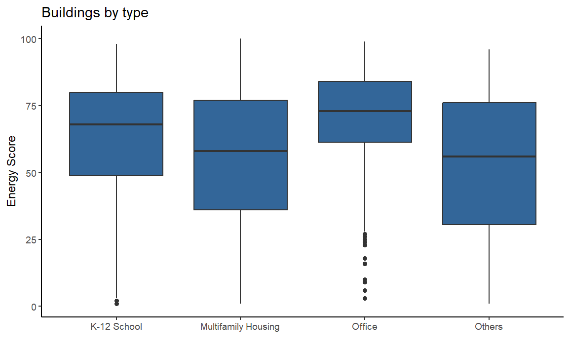
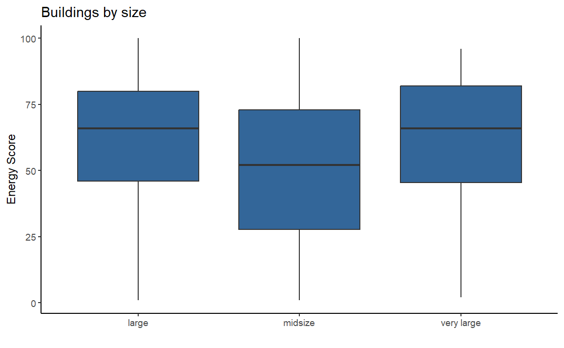
We review if the Energy Score changes depending on type of the houses and their sizes, Specifically, we found that multifamily houses and midsize buildings tend to have a lower energy score compared to other types and sizes of buildings.
clean_ny <- clean_ny %>%
  mutate(type = if_else(type %in% c("Multifamily Housing"),
                                    "Multifamily Housing",
                      if_else(type %in% c("K-12 School"), "K-12 School",
                              if_else(type %in% c("Office"), "Office",
                              "Others"))))   %>%
  mutate(area = case_when(
    area <= 50000 ~ "midsize",
    area > 50000 & area <= 500000 ~ "large",
    area > 500000 ~ "very large",
  )) %>% mutate(area=as.factor(area))

clean_ny %>% ggplot(aes(type, energy_score)) +
  geom_boxplot(fill="#336699") +
  labs(title= "Buildings by type", y="Energy Score", x="") +
  theme_classic()
clean_ny %>% ggplot(aes(area, energy_score)) +
  geom_boxplot(fill="#336699") +
  labs(title= "Buildings by size",  y="Energy Score", x="") +
  theme_classic()
Removing outliers
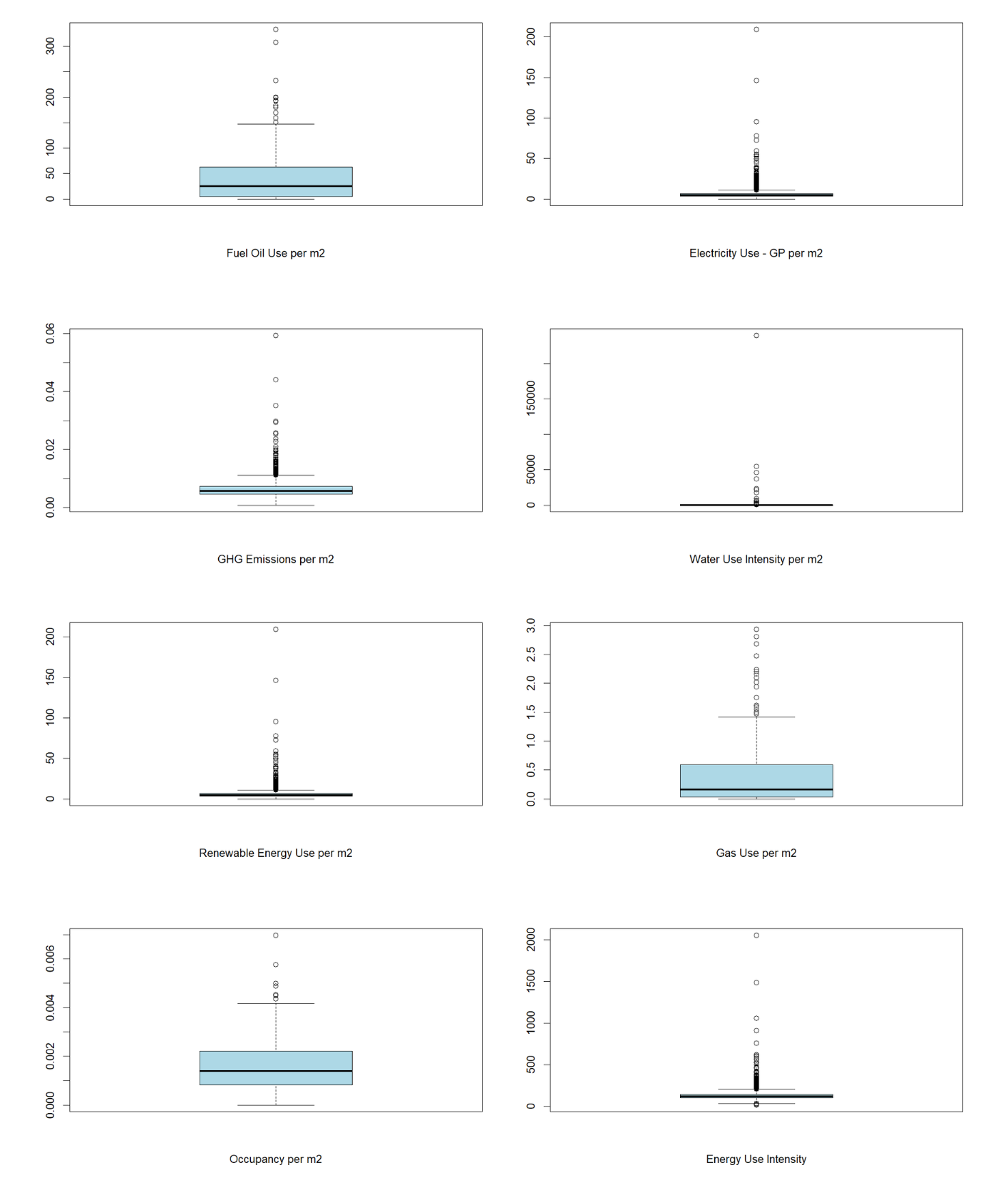
The boxplots depicted below indicate the presence of numerous outliers in the majority of variables. To address this, we utilize the Interquartile Range Rule and remove the outliers from the dataset.
boxplot(clean_ny$occupancy_pa, xlab="Occupancy per m2", col="lightblue")
boxplot(clean_ny$eui, xlab="Energy Use Intensity", col="lightblue")
boxplot(clean_ny$ghg_emissions_pa, xlab="GHG Emissions per m2", col="lightblue")
boxplot(clean_ny$fueloil_use_pa, xlab="Fuel Oil Use per m2", col="lightblue")
boxplot(clean_ny$gas_use_pa, xlab="Gas Use per m2", col="lightblue")
boxplot(clean_ny$electricity_useGP_pa, xlab="Electricity Use - GP per m2", col="lightblue")
boxplot(clean_ny$renewables_use_pa, xlab="Renewable Energy Use per m2", col="lightblue")
boxplot(clean_ny$wui, xlab="Water Use Intensity per m2", col="lightblue")
detect_outliers = function(x){
  q1 = quantile(x, probs=.25)
  q3 = quantile(x, probs=.75)
  iqr = q3-q1
  x > (q3 + (iqr*1.5)) | x < (q1-(iqr*1.5) )
}

rmv_outliers = function(dataframe, columns=names(dataframe)) {
    for (col in columns) {
        dataframe <- dataframe[!detect_outliers(dataframe[[col]]), ]
    }
    dataframe
}

buildings_clean = rmv_outliers(clean_ny, c("occupancy_pa", "eui",
          "fueloil_use_pa","gas_use_pa","electricity_useGP_pa",
          "renewables_use_pa","ghg_emissions_pa","wui" ))
# Select continuous variables
ny_buildings = buildings_clean %>% select(!c(Property.Id,type, Latitude,
Longitude, area))
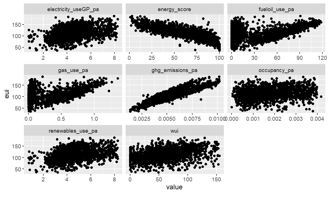
plot_scatterplot(ny_buildings, by="eui")
Correlations
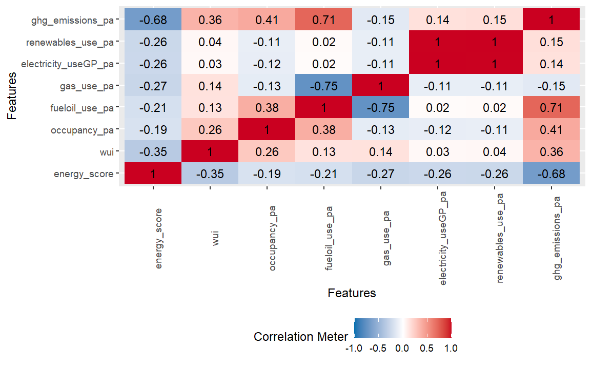
The analysis of the correlations reveals that most of our predictors are negatively correlated with the energy score, suggesting as hypothesis that higher resource consumption is associated with lower energy efficiency. We also detected multicollinearity between the variables of renewable energy use and electricity use from the grid. These variables measure similar characteristics in terms of energy consumption and have a perfect correlation, leading us to discard the renewable energy variable.
plot_correlation(ny_buildings %>% select(!eui))
Target variable
ny_buildings = buildings_clean %>% select(!c(Property.Id))
ny_buildings = ny_buildings %>% mutate(
  efficiency = as.factor(ifelse(energy_score > 75, "Yes", "No"))
) %>% select(!energy_score)
3. Modeling
Train-test split
set.seed(163)
# split data
in_train <- createDataPartition(ny_buildings$efficiency, p = 0.75, list = FALSE)
training <- ny_buildings[in_train,]
testing <- ny_buildings[-in_train,]
Cross validation (10 folds)
ctrl = trainControl(
  method = "repeatedcv",
  number = 10,
  classProbs = T,
  summaryFunction = twoClassSummary,
  verboseIter = T
  )
Training Logistic Regression
We chose to begin with a logistic regression model because it enables us to model the probability of a binary target variable, and its results are highly interpretable.
logistic = train(
  efficiency ~
    area+wui+occupancy_pa+fueloil_use_pa+gas_use_pa+electricity_useGP_pa+
    ghg_emissions_pa+type,
  data = training,
  method= "glm",
  family = "binomial",
  metric = "ROC",
  preProc= c('scale', 'center'),
  tuneLength= 10,
  trControl = ctrl)

#model summary
tab_model(logistic$finalModel)
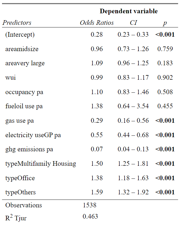
Out of the total variables considered, we found 7 variables to be statistically significant in predicting energy efficiency. Among these variables, GHG emissions and gas use were found to have a strong negative association with the probability of a building being energy-efficient.
Evaluation
log_prediction <- predict(logistic,testing,type="prob")
prediction = as.factor(ifelse(log_prediction[,2]>0.5, "Yes", "No"))

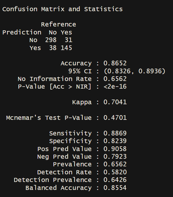
confusionMatrix(prediction, testing$efficiency)
roc(testing$efficiency, log_prediction[,2])$auc
Area under the curve: 0.9229
The model’s performance metrics are satisfactory, but we would like to explore an alternative machine learning model to investigate if other non-linear variables, such as longitude and latitude, could affect the results.
Fit Random Forest
rfFit = train(
  efficiency ~
    area+wui+occupancy_pa+fueloil_use_pa+gas_use_pa+electricity_useGP_pa+
    ghg_emissions_pa+type+Longitude+Latitude,
  data = training,
  method= "rf",
  preProc= c('scale', 'center'),
  tuneLength= 10,
  metric = "ROC",
  trControl = ctrl
)
rfProb = predict(rfFit, testing, type = "prob")
prediction = as.factor(ifelse(rfProb[,2]>0.5, "Yes", "No"))

confusionMatrix(prediction, testing$efficiency)
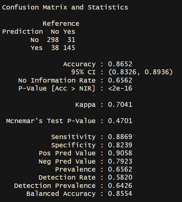
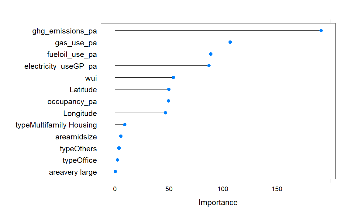
After comparing the results of the logistic regression and the machine learning model, we found that the predictions are not significantly affected by the inclusion of non-linear variables such as longitude and latitude. However, we still wanted to assess the importance of variables for prediction and evaluate the AUC to gain a better understanding of the model’s performance.
plot(varImp(rfFit, scale = F), scales = list(y = list(cex = .95)))
roc(testing$efficiency, rfProb[,2])$auc
Area under the curve: 0.9426
4. Conclussions
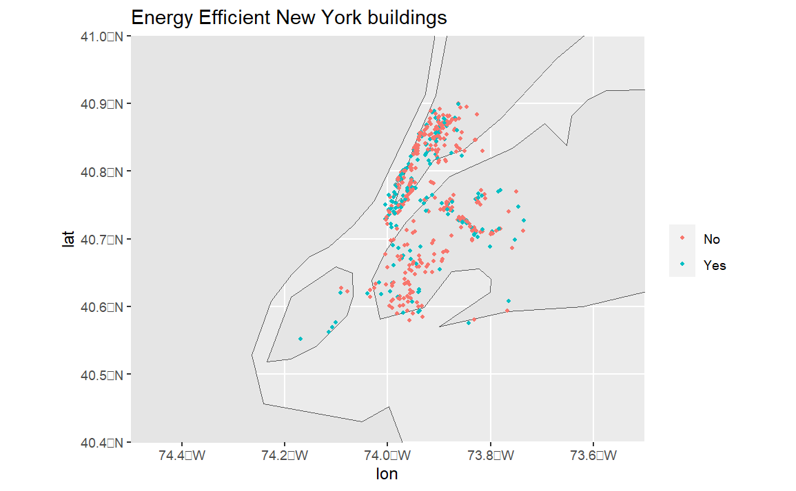
We have confirmed that buildings that consume more resources are less likely to be energy-efficient, and our predictions have been highly accurate. Our models have provided different approaches to the problem at hand. The logistic regression model has shown the clear effect of predictors on our response variable. The random forest model increased the AUC, but didn’t significantly improve other performance metrics. Finally, we have visualized the geographical distribution of energy-efficient buildings in NYC.
world <- ne_countries(scale = "medium", returnclass = "sf")

sites <- data.frame(lon = testing$Longitude, lat= testing$Latitude, efficiency=prediction)

ggplot(data = world) +
    geom_sf() +
    geom_point(data = sites, aes(x = lon, y = lat, color=factor(efficiency)),
    size = 1) +
    coord_sf(xlim = c(-73.5, -74.5), ylim = c(40.4, 41), expand = FALSE) +
  ggtitle("Energy Efficient New York buildings") +
  labs(color = "Energy Efficiency")
